Equations of Motion
Graphical Analysis of Motion
Before we derive the equations, we must understand how to interpret motion through graphs. These are the visual foundations of kinematics.Graphical representation of motion is crucial to understand different types of motion ,including uniform motion,nonuniform motion,acceleration and de-acceleration.
Position-Time (x-t) Graph
In position / Time graph the X-axis represents the Time and Y – Axis represents the displacement (Change in position)
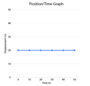
1. Object at rest
When an object at rest means stationary, its position does not change with time.Hence change in displacement is Zero and its velocity is Zero. V = X2 – X1/T2 – T1
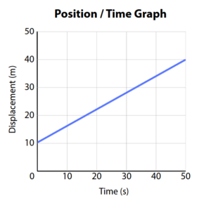
2. Object moving with a constant velocity (Uniform motion)
Let s say, A car travels equal distance in equal interval of time,then its velocity is constant.A constant velocity can be positive or negative based on the direction of the car.when we plot the position / time graph we’ll get a straight line as shown below in the image.
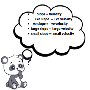
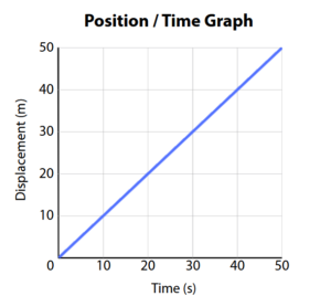 Slope of the graph = Velocity of the car
From the slope, one can also predict whether the car is traveling fast or slow.
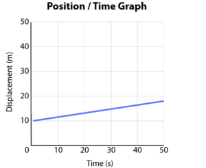
Positive (Fast) Positive (Slow)
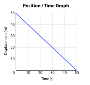
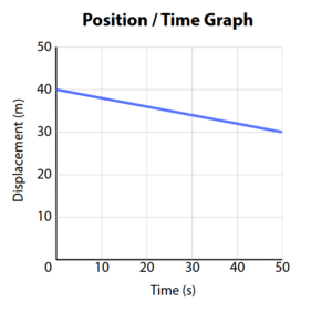
Negative (fast) Negative (Slow)
- This graph helps to understand velocity and types of motion.
- Slope: Represents the Velocity of the object.

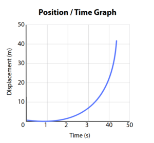
3. Object moving with a changing velocity (Nonuniform Motion)
when the car coves unequal distance in equal interval of time , meaning its velocity changes (nonuniform motion), the car is accelerating.If the position /time graph were plotted for such motion the resulting graph would be a curved line as shown in the image below.
Velocity-Time (v-t) Graph
[PLACEHOLDER: INSERT VELOCITY-TIME GRAPH IMAGE HERE]
- Slope: Represents the Acceleration.
- Area under the curve: Represents the Displacement (change in position).
The Four Equations of Motion
These equations apply only when acceleration is constant. We use the following symbols:
- u: Initial Velocity
- v: Final Velocity
- a: Constant Acceleration
- t: Time Interval
- s: Displacement
Equation 1: The Velocity Equation
v = u + at
Derivation: By definition, acceleration (a) is the rate of change of velocity.
a = (v – u) / t
Multiply both sides by t: at = v – u
Rearrange: v = u + at
Equation 2: The Displacement Equation
s = ut + (1/2)at²
Derivation: Displacement is the area under a v-t graph. For constant acceleration, this area is a trapezoid (or a rectangle + triangle).
Area = (u * t) + 1/2 * (base * height)
Area = ut + 1/2 * (t) * (v – u)
Since (v – u) = at, substitute it in:
s = ut + 1/2at²
Equation 3: The Timeless Equation
v² = u² + 2as
Derivation: Start with v = u + at and solve for t: t = (v – u) / a.
Substitute this t into the displacement formula s = ((u + v) / 2) * t.
s = ((u + v) / 2) * ((v – u) / a)
2as = (v + u)(v – u)
2as = v² – u²
Rearrange: v² = u² + 2as
Equation 4: Average Velocity Displacement
s = [(u + v) / 2] * t
Explanation: This equation shows that displacement is simply the average of the initial and final velocities multiplied by time.
Example Problem: The Braking Car
Problem: A car traveling at 30 m/s applies its brakes and comes to a complete stop in 6 seconds. Calculate the acceleration and the total distance covered during braking.
1. Identify the Givens:
- Initial Velocity (u) = 30 m/s
- Final Velocity (v) = 0 m/s (since it stops)
- Time (t) = 6 s
2. Find Acceleration (a):
Using v = u + at:
0 = 30 + a(6)
-30 = 6a
a = -5 m/s² (The negative sign indicates deceleration)
3. Find Displacement (s):
Using s = ut + 1/2at²:
s = (30)(6) + 1/2(-5)(6²)
s = 180 + 1/2(-5)(36)
s = 180 – 90
s = 90 meters
Conclusion: The car decelerates at 5 m/s² and takes 90 meters to stop.