Understanding Position-Time (x-t) Graphs
Before deriving the fundamental equations of motion, it is essential to master the interpretation of motion through graphical analysis. Position-time graphs provide a visual representation that is crucial for distinguishing between various states of motion, such as uniform and non-uniform movement.
In a standard position-time graph, the horizontal X-axis represents the progression of Time, while the vertical Y-axis represents the object’s Displacement or change in position.
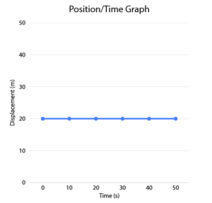
1. Object at Rest
When an object is stationary, its position remains constant regardless of the passage of time. In this state, the velocity is zero, which is represented mathematically as:
V = (X₂ – X₁) / (T₂ – T₁) = 0
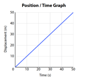
2. Uniform Motion (Constant Velocity)
Uniform motion occurs when an object covers equal distances in equal intervals of time, resulting in a straight, sloped line. The steepness or slope of this line directly represents the object’s velocity.
Velocity Comparison and Direction
The direction and magnitude of velocity can be determined by observing the orientation and steepness of the slope.
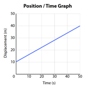 Positive (Fast): A steep upward slope indicating high velocity in the positive direction.
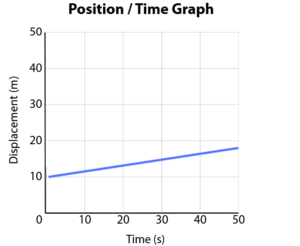 Positive (Slow): A gentle upward slope indicating low velocity in the positive direction.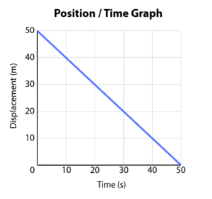
Negative (Fast): A steep downward slope representing high velocity in the opposite direction.
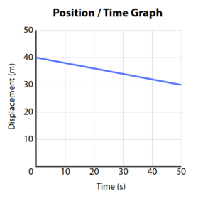
Negative (Slow): A gentle downward slope representing low velocity in the opposite direction.
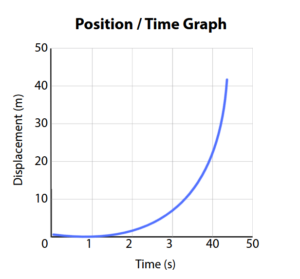
3. Non-Uniform Motion (Acceleration)
When an object covers unequal distances in equal time intervals, its velocity is changing. On a position-time graph, this acceleration is visualized as a curved line, indicating that the slope (velocity) is not constant.